How I Built an Instrument for CPC Expansion
A simulated IV approach validated with Monte Carlo evidence
 Monte Carlo validation of the simulated IV strategy
The core empirical challenge in studying crisis pregnancy centers is familiar to any applied economist: selection on unobservables. CPCs do not open randomly. They tend to locate in areas with larger populations, more religious institutions, and potentially higher abortion rates. A naive regression of abortion rates on CPC counts would be biased. In fact, OLS understates the causal effect because CPCs locate where abortion demand is high for unobserved reasons, attenuating the estimate toward zero.
This post explains the simulated instrumental variables (IV) strategy I developed for my paper and shows Monte Carlo evidence that it works.
The idea
Simulated instruments have a long history in economics, dating back to Currie and Gruber (1996) on Medicaid eligibility. The core logic is to generate predicted exposure from predetermined characteristics that is plausibly exogenous to local shocks. My approach extends this to a dynamic, path-dependent setting, connecting to the formula instruments framework of Borusyak, Hull, and Jaravel (2025).
CPC expansion is not driven by discrete policy shocks or regulatory discontinuities. It is a decentralized process where individual organizations respond to local conditions over decades. The probability that a county receives its kth CPC depends on the entire history of past placements, compounding over 30 years into a nonlinear function of past observables and organizational shocks. No standard difference-in-differences design works here. The instrument construction proceeds in two steps.
Step 1: Hazard model. I estimate a discrete-time logit of CPC entry, where the probability of a new CPC opening in county c at time t depends on predetermined county characteristics: lagged CPC stock, distance to the nearest CPC, lagged abortion rates, abortion provider presence, demographics, religious composition, political ideology, unemployment, county fixed effects, and a polynomial time trend. Counties can receive multiple CPCs; the model allows repeated events by conditioning on accumulated stock.
Step 2: Forward simulation. Starting from observed 1990 conditions, I forward-simulate 1,000 counterfactual CPC expansion paths. Each draw uses independent random shocks and the predicted opening probabilities to determine CPC entry, updating county characteristics (CPC stock, distance to nearest CPC) recursively each year. Averaging simulated CPC presence across draws yields the instrument, which converges to the conditional expectation of CPC presence given predetermined characteristics. The simulation is a computational device: the random shocks are computer-generated numbers, and averaging 1,000 draws eliminates them by the law of large numbers, leaving a deterministic function of the lagged observables.
The identifying assumption is predetermination: conditional on rich historical observables and two-way fixed effects, the residual timing of CPC openings is orthogonal to contemporaneous fertility shocks. The exclusion restriction follows from the law of iterated expectations, without requiring a separate argument about the instrument’s channels of influence. The hazard model determines instrument strength (first-stage F = 170) and complier weighting, not the exclusion restriction. Misspecifying the hazard weakens the first stage but does not introduce bias as long as predetermination holds.
Monte Carlo validation
The Monte Carlo exercise validates the estimator under severe designed endogeneity. The design crosses three true treatment effects (beta = -0.10, -0.20, -0.30) with three data-generating processes, for nine cells with 100 replications each. Crucially, the hazard model is deliberately misspecified in all cells: the true DGP includes confounders and functional forms not available to the hazard estimator, so the instrument is constructed from a model the researcher knows is wrong.
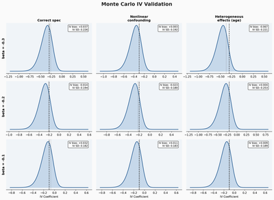
The figure shows results across a 3x3 grid. The rows correspond to three true effect sizes (beta = -0.30, -0.20, -0.10). The columns correspond to three data-generating processes of increasing complexity.
Additive confounding (left column). The DGP includes an additive confounder that drives both CPC placement and outcomes. OLS is severely biased, with mean estimates near +1.5 when the true effect is negative, a sign reversal. The IV recovers the truth with small bias.
Nonlinear confounding (middle column). The confounder enters through an interaction with treatment, which the linear model cannot capture. The IV still performs well. Bias remains small, confirming that the instrument is robust to this form of misspecification.
Heterogeneous effects by age (right column). The treatment effect varies across age groups, and the instrument recovers a weighted average. Bias is small across all three true effect sizes. The variance is somewhat larger, which is expected when the instrument captures an average of heterogeneous effects.
Across all nine cells, the IV bias never exceeds 0.07 in absolute value, and 95% confidence interval coverage is near nominal. This is not a proof that the instrument works in the real data, but it establishes that the statistical machinery recovers the right number even when the hazard model is wrong, confirming that instrument validity depends on predetermination, not on correct specification of the hazard.
What the Monte Carlo does not do
It doesn’t validate the identifying assumption itself. If predetermination fails, say because CPC openings were anticipated and triggered behavioral responses before the CPC appeared, or because CPC entry coincided with abortion clinic closures for reasons the instrument cannot capture, the IV could still be biased. The paper addresses these concerns with event study pre-trend tests (flat for abortion, birth, and pregnancy), a permutation test shuffling the instrument across counties (first-stage F of 0.69 vs. 170 in the actual data), and sensitivity to alternative specifications.
The value of the Monte Carlo is narrower: given predetermination, the estimator recovers the right number even when the hazard model is deliberately wrong.
Why show this?
Most applied papers assert instrument validity with a first-stage F-statistic and a plausibility argument. Monte Carlo validation goes further by demonstrating the estimator’s performance under controlled conditions where the answer is known. For simulated instruments, where the prediction step introduces additional degrees of freedom, this kind of exercise is especially valuable. It takes a few hours to code and can reveal problems that no amount of hand-waving about the exclusion restriction will catch.
For context on the CPC setting and expansion patterns, see How Crisis Pregnancy Centers Spread Across the Carolinas. For the age-specific results this instrument produces, see Who Do Crisis Pregnancy Centers Actually Affect?